
This is my notes of the course “MITx: 18.6501x Fundamentals of Statistics” on edX. The session that I participated started on Sept 2, 2019. The purpose of this document is to help me remember what I have learnt.
Here is the link of the course.
Note: a site to calculate/look up statistic curves/values: link
Unit 1: Introduction to Statistics
Probability and Statistics
Very explicit explanation of the relation of probability and statistics:
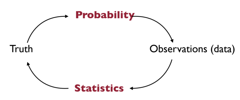
If we know the truth, then we can use “Probability” to predict/explain the “Observations”. However,
statistics is reverse engineering probability.
We have some observations (most of time we call them data), but we have no idea about the truth. We use the observations to estimate the truth. This is the purpose of statistics. From data, we try to recover what the truth is like.
Some conceptions
i.i.d.
Data that i.i.d. stands for independent and identically distributed .
A collection of random variables $X_1,…,X_n$ are i.i.d. if
- each $X_i$ follows a distribution $P_i$, all those distributions $P_i$ are the same, and
- $X_i$ are (mutually) independent
Sample average
We denote the sample average, or sample mean, of n random variables $X_1,…,X_n$ by
\[\bar X_n=\frac 1n\sum _{i=1}^nX_i\]Laws of Large Numbers (LLN)
Let $X_1,X_2,…,X_n$ be i.i.d. random variables, with $\mu=E[X]$ and $σ^2=Var[X]$.
Laws (weak and strong) of large numbers (LLN):
\[\bar X_n = \frac 1n\sum _{i=1}^nX_i\xrightarrow[n\to \infty]{P,\; a.s.}\mu\]where the convergence is in probability (as denoted by P on the convergence arrow) and almost surely (as denoted by a.s. on the arrow) for the weak and strong laws respectively.
When n is large enough, the sample average will converge to the expectation of variables.
Central Limit Theorem (CLT)
\[\sqrt n \frac {\bar X_n-\mu}{\sigma}\xrightarrow [n\to \infty]{(d)}\mathcal{N}(0,1) \\ \quad \\ \text {or:}\quad \sqrt n (\bar X_n-\mu)\xrightarrow [n\to \infty]{(d)}\mathcal{N}(0,\sigma^2)\]where the convergence is in distribution, as denoted by (d) on top of the convergence arrow.
Rule of thumb: n $\geq$ 30, to use CTL.
When n is large enough, the sample average converges to a Gaussian distribution.
Three inequalities
Hoeffding’s Inequality
When n is not large enough to apply CTL, we can use Hoeffding’s Inequality.
Given n (n>0) i.i.d. random variables $X_1,X_2,\ldots ,X_ n\stackrel{iid}{\sim }X$ that are almost surely bounded, meaning $\mathbf{P}(X\notin [a,b]=0$.
\[\mathbf{P}\left(\left|\overline{X}_ n-\mathbb E[X]\right|\geq \epsilon \right) \leq 2 \exp \left(-\frac{2n\epsilon ^2}{(b-a)^2}\right)\quad \text {for all }\epsilon >0.\]Unlike for the central limit theorem, here the sample size n does not need to be large.
Markov inequality
For a random variable $X\geq 0$ with mean $\mu>0$, and any number $t>0$:
\[\mathbf {P}(X\geq t) \leq \frac {\mu}{t}\]Note that the Markov inequality is restricted to non-negative random variables.
Chebyshev inequality
For a random variable X with (finite) mean $\mu$ and variance $\sigma^2$, and for any number $t\geq0$,
\[\mathbf{P}\left(\left|X-\mu \right|\geq t\right)\leq \frac{\sigma ^2}{t^2}\]When Markov inequality is applied to $(X-\mu)^2$, we obtain Chebyshev’s inequality. Markov inequality is also used in the proof of Hoeffding’s inequality.
Gaussian distribution
It is named after German Mathematician Carl Friedrich Gauss (1777–1855) in the context of the method of least squares (regression).
Gaussian density (PDF)
\[f_{\mu,\sigma^2}(x)=\frac{1}{\sigma \sqrt{2\pi }} \exp \left(-\frac{(x-\mu )^2}{2 \sigma ^2}\right)\]There is no closed form for their cumulative distribution function (CDF).
Useful properties of Gaussian
Invariant under affine transformation
$X\sim \mathcal{N}(\mu,\sigma^2)$, then for any $a,b \in \mathbb {R}$,
\[aX+b \sim \mathcal{N}(a\mu+b,a^2\sigma^2)\]Standardization
a.k.a. Normalization/Z-score. If $X\sim \mathcal{N}(\mu,\sigma^2)$, then
\[Z=\frac {X-\mu}{\sigma} \sim \mathcal{N}(0,1)\]Useful to compute probabilities from CDF of $Z\sim\mathcal{N}(0,1)$:
\[\mathbf {P}(u\leq X \leq v)=\mathbf {P}(\frac {u-\mu}{\sigma}\leq Z \leq \frac {v-\mu}{\sigma})\]Symmetry
if $X\sim \mathcal{N}(0,\sigma^2)$ and $x>0$:
\[\mathbf {P}(|X|> x)=2\mathbf {P}(X> x)\]Quantiles
Let $\alpha$ in (0,1), the quantile of order $1-\alpha$ of a random variable $X$ is the number $q_\alpha$ such that:
\[\mathbf{P}\left(X\leq q_{\alpha }\right)=1-\alpha\]Let $F$ denote the CDF of $X$:
- $F(q_{\alpha })=1-\alpha$
- if $F$ is invertible, then $q_{\alpha }=F^{-1}(1-\alpha)$
- $\mathbf{P}\left(X> q_{\alpha }\right)=\alpha$
- if $X \sim \mathcal N(0,1)$, then $\mathbf P \vert x \vert > q_ {\alpha/2}=\alpha$
Some important quantiles of the $Z\sim \mathcal{N}(0,1)$ are:
| $\alpha$ | 2.5% | 5% | 10% |
|---|---|---|---|
| $q_{\alpha}$ | 1.96 | 1.65 | 1.28 |
Three types of convergence
- $(T_n)_{n\geq 1}$ is a sequence of random variables
- T is a random variable (T may be deterministic)
Almost surely (a.s.) convergence
is also known as convergence with probability 1 (w.p.1) and strong convergence.
\[T_ n\xrightarrow [n\rightarrow \infty ]{a.s.}T \quad \text {iff} \quad \mathbf P[\{ \omega : T_n\xrightarrow [n\rightarrow \infty ]{}T(\omega)\}]=1\]Convergence in probability
\[T_ n\xrightarrow [n\rightarrow \infty ]{\mathbf P}T \quad \text {iff} \quad \mathbf P[|T_n-T|\geq \epsilon]\xrightarrow [n\rightarrow \infty ]{}0,\forall\epsilon >0\]Convergence in distribution
is also known as convergence in law and weak convergence .
\[T_ n\xrightarrow [n\rightarrow \infty ]{(d)}T \quad \text {iff} \quad \mathbb E[f(T_ n)]\xrightarrow [n\rightarrow \infty ]{}\mathbb E[f(T)]\]for all continuous and bounded function $f$.
When n is large enough, they have the same distribution (the same PDF/CDF).
Properties
- If $(T_n)_{n\geq 1}$ converges a.s., then it also converges in probability, and the two limits are equal a.s.
- If $(T_n)_{n\geq 1}$ converges in probability, then it also converges in distribution
-
Convergence in distribution implies convergence of probabilities if the limit has a density (e.g. Gaussian):
\[T_ n\xrightarrow [n\rightarrow \infty ]{(d)}T \Rightarrow \mathbf {P}(a\leq T_n \leq b)\xrightarrow [n\rightarrow \infty ]{}\mathbf {P}(a\leq T \leq b)\] -
Addition, Multiplication, and Division preserves convergence almost surely (a.s.) and in probability ($\mathbf P$)
More precisely, assume
\[T_ n\xrightarrow [n\rightarrow \infty ]{a.s. /\mathbf P}T \quad \text {and} \quad U_ n\xrightarrow [n\rightarrow \infty ]{a.s. /\mathbf P}U\]Then,
- $T_ n+U_n\xrightarrow [n\rightarrow \infty ]{a.s. /\mathbf P}T+U$
- $T_ nU_n\xrightarrow [n\rightarrow \infty ]{a.s. /\mathbf P}TU$
- if in addition, $U\ne0$ a.s., then $\frac {T_ n}{U_n}\xrightarrow [n\rightarrow \infty ]{a.s. /\mathbf P}\frac {T}{U}$
In general, these rules do not apply to convergence in distribution (d).
Slutsky’s Theorem
For convergence in distribution, the Slutsky’s Theorem will be our main tool.
Let $(T_ n), (U_ n)$ be two sequences of r.v., such that:
- $T_ n\xrightarrow [n\to \infty ]{(d)}T$
- $U_ n\xrightarrow [n\to \infty ]{\mathbf{P}}u$
where $T$ is a r.v. and $u$ is a given real number (deterministic limit: $\mathbf{P}(U=u)=1$). Then,
- $T_ n+U_n\xrightarrow [n\rightarrow \infty ]{(d)}T+u$
- $T_ nU_n\xrightarrow [n\rightarrow \infty ]{(d)}Tu$
- if in addition, $u\ne0$ a.s., then $\frac {T_ n}{U_n}\xrightarrow [n\rightarrow \infty ]{(d)}\frac {T}{u}$
Continuous Mapping Theorem
If $f$ is a continuous function:
\[T_ n\xrightarrow [n\rightarrow \infty ]{a.s./\mathbf P/(d)}T \Rightarrow f(T_n) \xrightarrow [n\rightarrow \infty ]{}f(T)\]